This short article seeks to describe how the Gumbel (or Type-1 Generalized Extreme Value) distribution’s use in probabilistic discrete choice models leads to a closed-form expression for choice probabilities.
A standard framework for a probabilistic discrete choice model (DCM) reflecting a random utility theory (RUT) in a cross-sectional setting is as follows:
- The utility that a decision maker obtains from alternative \(j\) is \(U_j\), for \(j = 1, \ldots, J\).
- The decision maker chooses the alternative that provides the greatest utility: choose alternative \(k\) if and only if \(U_k > U_j \hspace{1ex} \forall j \ne k\).
- Utility is decomposed to reflect the researcher’s inability to understand or observe all factors that impact choices: \(U_j = V_j + \varepsilon_j\) where the joint density of the random vector \(\mathbf{\varepsilon} = (\varepsilon_1, \ldots, \varepsilon_J)\) for the decision maker is \(f_\mathbf{\varepsilon}(\mathbf{\varepsilon})\).
The probability that the decision maker chooses alternative \(k\) is:
\[\begin{align*} P_{k} &= \text{Prob}\left( U_k > U_j \; \forall j \ne k \right) &\\ &= \text{Prob}\left( V_k + \varepsilon_k > V_j + \varepsilon_j \; \forall j \ne k \right) &\\ &= \text{Prob}\left( \varepsilon_j < \varepsilon_k + V_k - V_j \; \forall j \ne k \right) &\\ \end{align*}\]
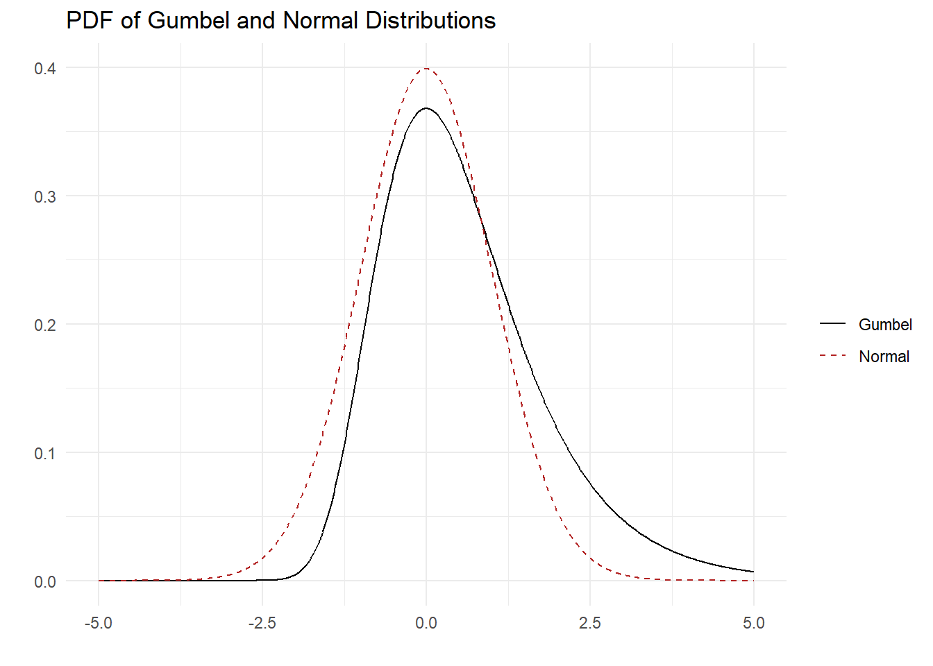
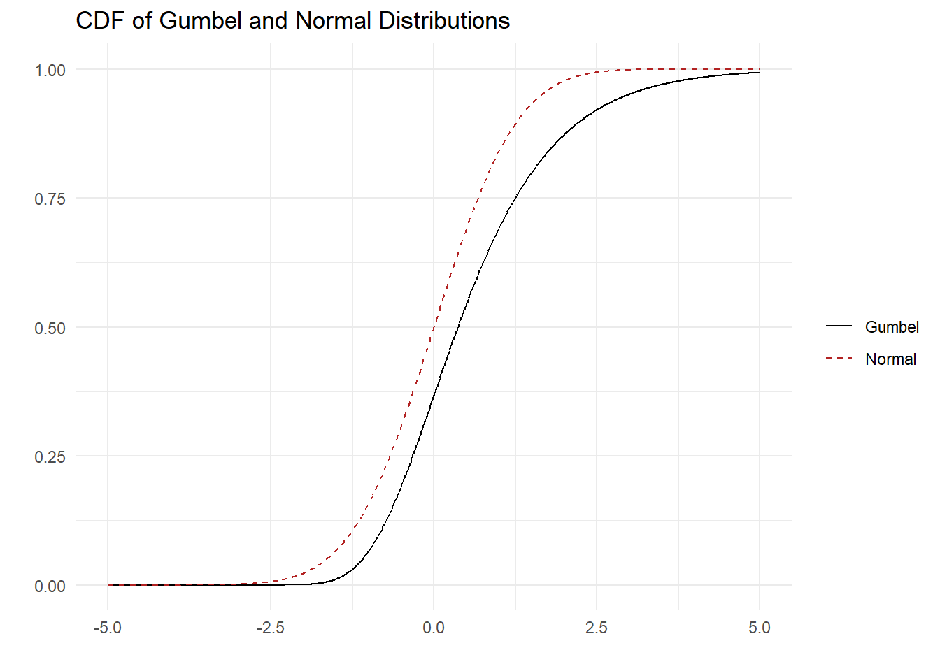
A common simplifying assumption about the joint distribution of vector \(\mathbf{\varepsilon}\) is that its components are independent and identically distributed as Gumbel random variables. Specifically, the cumulative distribution function for each \(\varepsilon_{j}\) is: \[ \text{Prob}(\varepsilon_j \leq x) = \exp(-\exp(-x)) = e^{-e^{-x}} \] The Gumbel density and distribution are plotted below (in black) alongside the Normal (in dashed red) for comparison.
Because each \(\varepsilon_j\) is assumed to be independently distributed, the probability that the decision maker chooses alternative \(k\) for a given value of \(\varepsilon_k\) can be written as the product of the \(J-1\) conditional distributions:
\[\begin{align*} P_k | \varepsilon_k &= \prod_{j \ne k} \exp(-\exp(-\varepsilon_k)) &\\ &= \exp \left( -\sum_{j \ne k} \exp \left( - ( \varepsilon_k + V_k - V_j) \right) \right) &\\ &= \exp \left( - \exp(\varepsilon_k) \times \sum_{j \ne k} \exp \left( V_j - V_k) \right) \right) \end{align*}\]
But of course \(\varepsilon_k\) is not given, so to obtain the desired probability \(P_k\), we must integrate over all possible values of \(\varepsilon_k\), weighted by its marginal density \(f_{\varepsilon_k}(\varepsilon_k) = \exp(-\varepsilon_k) \times \exp \left( -\exp(\varepsilon_k) \right)\): \[ P_k = \int_{-\infty}^{\infty} \exp(-\varepsilon_k) \times \exp \left( - \exp(\varepsilon_k) \times \sum_{j=1}^J \exp \left( V_j - V_k) \right) \right) \, d \varepsilon_k \]
For notational simplicity, denote \(a = \sum_{j=1}^J \exp ( V_j - V_k)\) and define the transformation of variables \(z = \exp(-\varepsilon_k)\). Then \(dz = -\exp(-\varepsilon_k) \, d \varepsilon_k = -z \, d \varepsilon_k\) and the integral becomes: \[ P_k = \int_\infty^0 z \times \exp ( - z \times a ) / (-z) \, dz = \int_0^\infty \exp (-z \times a ) \, dz \]
Evaluating the integral yields: \[ P_k = - \left[ \frac{1}{a} \times \left( 0-1 \right) \right] = \frac{1}{a} = \frac{1}{\sum_{j=1}^J \exp(V_j-V_k)} = \frac{\exp(V_k)}{\sum_{j=1}^J \exp(V_j)} \]
This is the familiar multinomial logit (MNL) choice probability.
Section 3.10 on page 74 of Kenneth Train’s book Discrete Choice Methods with Simulation provides a related derivation. If you are reading this post but have not yet read Train’s book, you should go read it now.